Enter this into the Superscope module:
|
Init
|
n = 50;
|
|
On Beat
|
|
|
Per Frame
|
|
|
Per Point
|
x = i*2-1-.5*v;
y = x+v;
y = -y;
|
The Breakdown
- n = 50;
- This sets the number of points to define at 50. The higher n is, the more detailed the scope is.
- x = i*2-1-.5*v;
- The first part of this equation (i*2-1) is used to stretch out the x values and shift them over to the left.
This is done because if we only use i, without multiplying or subtracting, we only get x-values between 0 and 1.
By multiplying by two and shifting it over one, we get values from -1 to 1, for the whole AVS Window. The second part, which
involves v, is merely to provide horizontal vibration in response to the music.
- y = x+v;
- This is the key part for defining the superscope to create a rectangular graph (which includes linear, quadratic,
polynomial, or sinusoidal functions). Where "y = x" appears in this equation is where one would place a rectangular
equation in this form.
examples:
- y = x
- is a linear function
- y = pow(x,2) [y = x squared]
- is a quadratic equation.
- y = pow(x,4) + 2*pow(x,3) + pow(x,2) + .5*x
- is a polynomial equation.
- y = sin(x)
- is a sinusoidal equation.
- y = log(x)
- is a logarithmic equation (natural log or log base e).
The +v is only for vibration of the scope, and doesn't play a part in defining the shape of the graph.
- y = -y;
- This inverts the y values so that they behave as they would if the top were 1 and the bottom were -1, instead of the
opposite (see the Window tutorial). This is essential to get the superscope to display the graph
of an equation as you expect it to be displayed.
Other Info
Along with this superscope module, don't forget to use a fadeout or blur from the +>Trans menu, or you'll end up with
little more than a white blob.
Some rectangular equations won't work with this format (circles, hyperbolas, and ellipses, for example). To create graphs
of these equations, one must use parametric equations and expand the i variable by using r. These will be addressed in future
tutorials.
Downloads
All 5 General Equation Types tutorials and demonstration AVS Presets.
Linear Equation tutorial and demonstration AVS Preset.
Quadratic Equation tutorial and demonstration AVS Preset.
Polynomial Equation tutorial and demonstration AVS Preset.
Sinusoidal Equation tutorial and demonstration AVS Preset.
Logarithmic Equation tutorial and demonstration AVS Preset.
|
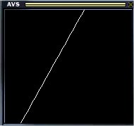
y = 2*x + 1
Linear

y = pow(x,2)
Quadratic
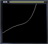
y = pow(x,4) + 2*pow(x,3) + pow(x,2) + .5*x
Polynomial
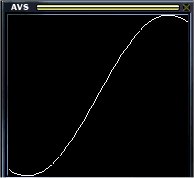
y = sin(2*x)
Sinusoidal
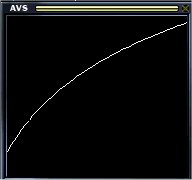
y = log(x+1.5)
Logarithmic
|